Job Openings and Labor Turnover Survey (JOLTS) Dataset
The Job Openings and Labor Turnover Survey (JOLTS) provides national estimates of rates and levels for various labor market dynamics. The survey covers job openings, hires, and total separations, further broken down into quits, layoffs and discharges, and other separations.
Dataset Files
The survey data is accessible through FTP files available in the BLS internet sub-directory pub/time.series/jt. These files include information on contacts, current data, all items, job openings, hires, total separations, quits, layoffs and discharges, other separations, and various mapping files providing additional context.
Series File
The jt.series file serves as a key component, detailing the structure and format of series identification codes. Each code includes information on seasonality, industry, state, area, size class, data element, rate level, and footnote codes. This information allows for precise identification and categorization of data series.
The JOLTS dataset is a valuable resource for understanding labor market dynamics, offering detailed and well-organized information that enables researchers, policymakers, and analysts to gain insights into the trends and patterns shaping the employment landscape.
2.2 Research Plan
Data Collection: As, the dataset is divide into different files, containing job openings, hires, separations, and industry specifics, we collect the files and convert into csv format for further analysis.
Preprocessing: Cleaning and organizing the data. Here we also analyse any missing values in our dataset.
Exploratory Analysis: Identify trends, patterns, and correlations in job data across industries and regions.
Addressing Research Questions: We merge our dataset files to uncover significant trends and relationships among various job analysis metrics. We plan to observe the following:
Industry Insights: Identify high-demand industries aligning with skills.
Job Market Trends: Analyze sectoral shifts over time for informed career choices.
Turnover Rates: Assess job stability and growth potential in different sectors.
Interactive component: Using D3, we provide engaging graphs to gain clear understanding on the dataset
Reporting: Summarize the findings, highlight insights, and present recommendations for career planning and job search strategies.
2.3 Missing value analysis
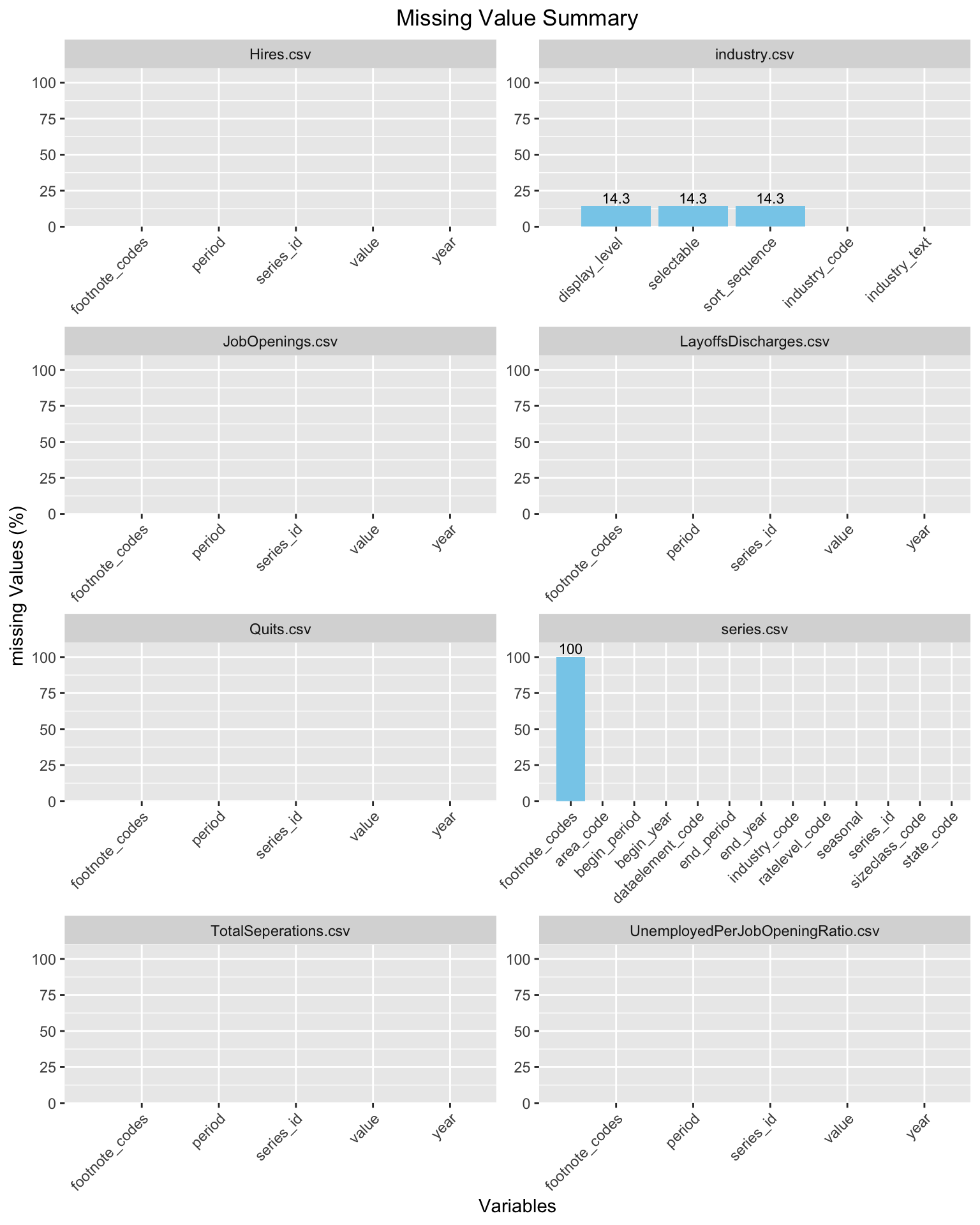
For most of our files we do not observe any missing values in the dataset. Majorly, the footnote_codes values are found to be missing in the datasets (wherever it referred). This may be due to the fact that this dataset only have 1 type of footnote which may be not linked to most of the data values. Particularly in the mapping files of industry dataset we observe display_level, selectable and sort_sequence to be missing from the dataset (in each 14.3% values are NA)
Code
suppressPackageStartupMessages({library(tidyverse)})folder_path <-"./data"csv_files <-list.files(folder_path, pattern ="\\.csv$", full.names =TRUE)all_missing_summary <-list()for (file in csv_files) { data <-read.csv(file) csv_file_name <-strsplit(file, "/")[[1]][3] missing_summary <- data %>%summarise_all(~mean(is.na(.)) *100) %>%gather(key ="variable", value ="missing_percentage") %>%arrange(desc(missing_percentage)) all_missing_summary[[csv_file_name]] <- missing_summary}combined_missing_summary <-bind_rows(all_missing_summary, .id ="csv_file_name")missing_value_graph <-ggplot(combined_missing_summary, aes(x =reorder(variable, -missing_percentage), y = missing_percentage)) +geom_bar(stat ="identity", fill ="skyblue") +geom_text(data =subset(combined_missing_summary, missing_percentage !=0),aes(label =round(missing_percentage, 1)), vjust =-0.3, size =3) +labs(title ="Missing Value Summary",x ="Variables",y ="missing Values (%)") +theme(axis.text.x =element_text(angle =45, hjust =1), plot.title=element_text(hjust=0.5)) +expand_limits(x =0, y =110) +scale_y_continuous(expand =c(0, 0)) +facet_wrap(~csv_file_name, scales ="free", ncol=2)print(missing_value_graph)
2.4 Missing Data Pattern
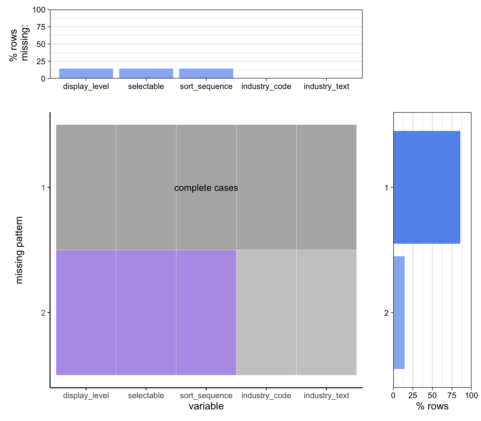
We observe that series.csv data only has one column which is missing for all the samples, on the other hand industry.csv has 3 columns which may have some pattern between the missing values. To further analyse this we use the redav package to identify the pattern in these missing values.
Scale for y is already present.
Adding another scale for y, which will replace the existing scale.
Scale for y is already present.
Adding another scale for y, which will replace the existing scale.
2.5 Data Summary
Code
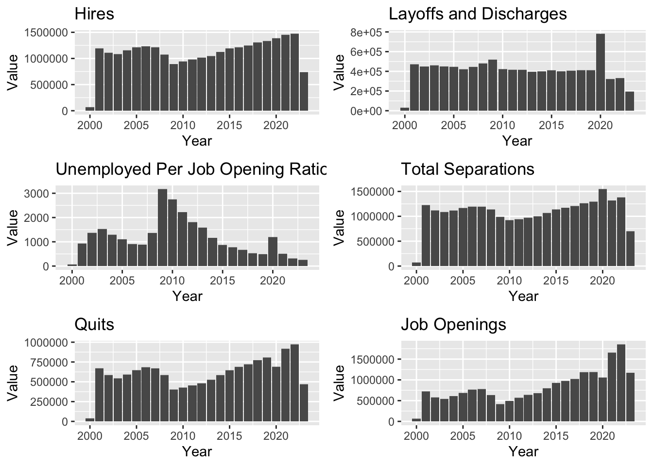
suppressPackageStartupMessages({library(ggplot2)library(tidyverse)library(gridExtra)})# Specify the folder pathfolder_path <-"./data/"# Read CSV files with full pathhires <-read.csv(paste0(folder_path, "Hires.csv"))layoffs_discharges <-read.csv(paste0(folder_path, "LayoffsDischarges.csv"))industry <-read.csv(paste0(folder_path, "industry.csv"))unemployed_per_job_opening_ratio <-read.csv(paste0(folder_path, "UnemployedPerJobOpeningRatio.csv"))total_separations <-read.csv(paste0(folder_path, "TotalSeperations.csv"))quits <-read.csv(paste0(folder_path, "Quits.csv"))job_openings <-read.csv(paste0(folder_path, "JobOpenings.csv"))series <-read.csv(paste0(folder_path, "series.csv"))create_histogram <-function(data, title, x_label, y_label) {suppressWarnings({ggplot(data, aes(x = year, y = value)) +geom_histogram(stat ="identity", bins =30, breaks =seq(min(data$year), max(data$year) +1, by =1)) +labs(title = title, x = x_label, y = y_label)})}# Create individual histogramshistogram_hires <-create_histogram(hires, "Hires", "Year", "Value")histogram_layoffs_discharges <-create_histogram(layoffs_discharges, "Layoffs and Discharges", "Year", "Value")histogram_unemployed_per_job_opening_ratio <-create_histogram(unemployed_per_job_opening_ratio, "Unemployed Per Job Opening Ratio", "Year", "Value")histogram_total_separations <-create_histogram(total_separations, "Total Separations", "Year", "Value")histogram_quits <-create_histogram(quits, "Quits", "Year", "Value")histogram_job_openings <-create_histogram(job_openings, "Job Openings", "Year", "Value")# Arrange histograms in a gridgrid.arrange( histogram_hires, histogram_layoffs_discharges, histogram_unemployed_per_job_opening_ratio, histogram_total_separations, histogram_quits, histogram_job_openings,ncol =2# Adjust the number of columns as per your preference)
From these graphs we see an dip in values around 2008, in Hires, Total Separations, Quits and Job Openings. And since then a gradual increase in value from 2008. The economic downturn in 2008 might expain the dip in numbers.
Another fascinating observation is the sudden spike in Layoffs and Discharges during the year 2019-2020. This can be attributed to the COVID-19 pandemic, when a lot of people lost their jobs.
A positive trend that one can observe is in the Unemployed Per Job Opening Ratio, which decreases from 2008, with the exception of the sudden spike in 2020, again due to COVID.